Excel and SQL Server Integration Service - PART I

In this blog we are going to discuss about how to load an EXCEL file using SSIS and how to do various transformation to the EXCEL files.

To do this I’m using SQL Server, Visual Studio 2012, SSDT and SSMS to store the tables. Basically this is an ETL approach. There are several other ways to export EXCEL files directly into a database using different tools as well. But in my agenda I’m going to use some different scenarios and complicated Excel files.

1. Excel Loading

Example 1

As a start first we’ll see how to load a simple EXCEL file.

Let’s say we have an EXCEL file with below structure. I have named this EXCEL sheet as “Semester_1”.

Now let’s load this EXCEL sheet into a database which created in SSMS and see the result. Following steps will help to achieve that.

First we have to create a database in the SSMS where we create the destination tables. I named it as Marks_DB.

Then we have to use SSIS package to build the ETL part. So, the ETL will look like below.

I have added a sequence container to hold the Execute SQL task which is used to truncate the destination table and a dataflow task where the operation will take place. There are two connection mangers where “Excel Connection Manager” created to connect to the EXCEL sheet and “Marks_DB” created to connect to the destination.

Tip 1: Tick “First row has column names” if you want to get the first row which available data as column headers.

Tip 2: If it gives an error as "SSIS Excel Connection Manager failed to Connect to the Source". Then installing 32-bit Microsoft Access Database Engine 2010 Redistributable will help to resolve the issue.

Now let’s have a look inside the dataflow task.

In here we have to set up and connect a source and a destination. Source is an Excel source and the destination is an OLE DB destination.

Excel source will be configured as below.

We have to choose the EXCEL connection manager which we created and the data access mode should be Table or view. Then select our EXCEL file from the “Name of the EXCEL sheet” list.

Then we can select preview where we can see the EXCEL sheet output.

Then we have to close the preview query result and select the columns from the EXCEL source editor.

Here we can see all the columns we going to extract from the Excel source file.

Then click ok and we done configuring the EXCEL source.

Now we have to configure the destination.

Finally, Run the package and after that we can see the destination in SSMS as below.

Example 2

Now let’s see how to load an EXCEL file with below structure. I have named this EXCEL sheet as “Semester_1”. 

As you can see there are two tables in the same Excel sheet. We have a vertical table and a horizontal table. We will first look in to the vertical table in this example and name the vertical table as Marks.

If we try to load the about EXCEL sheet as we did in Example 1 we’ll end up getting an output like below.

As you can see in the above image this is not the exact output we need.

To get the marks table as output we can follow two methods.

Method 1 – Data Access Mode as Table or view

After we setup the EXCEL source with the EXCEL sheet we’ll have a preview of source data like below.

Then go to the columns and you’ll see something like below.

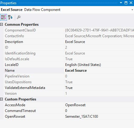
Now click ok. Then right click and select properties of the EXCEL source and change the Open row set as below to define the EXCEL sheet area which we need to read.

Then again open and check the EXCEL source and you’ll able to see the Connection Manager, preview and Columns as below.

Now we can do same as Example 1 to load the destination and the final destination output will look like below.

Method 2 – Data Access Mode as SQL command

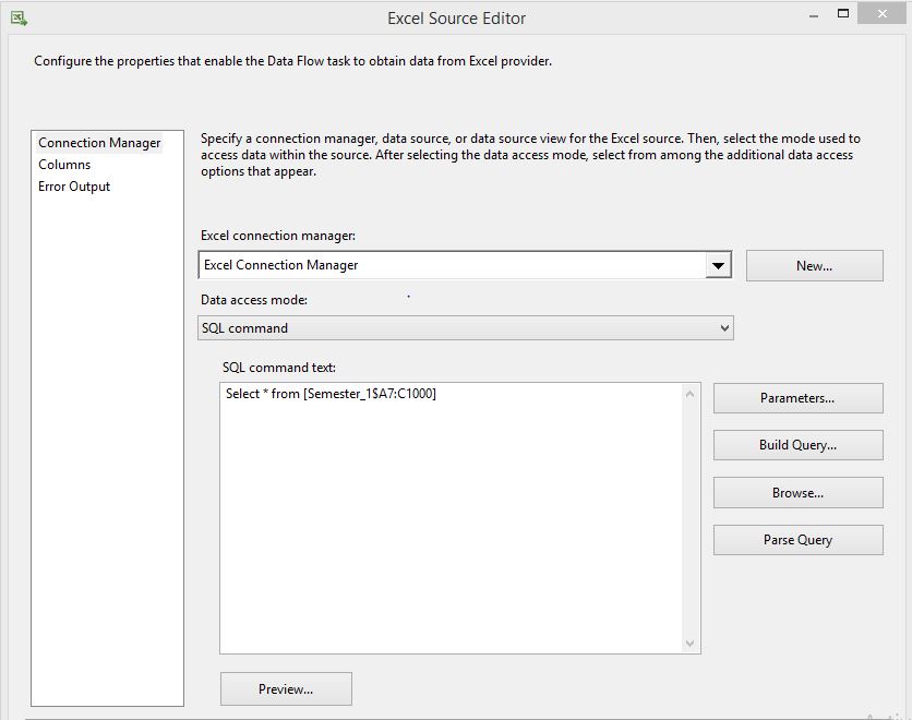
In this method after selecting the connection manager in the EXCEL source we need to change the Data Access Mode to SQL command and type the SELECT query with the EXCEL sheet and mention the area to consider as below.

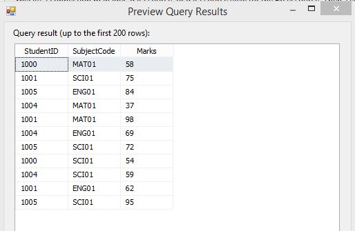
Then we’ll get the preview and columns of the EXCEL source as below.

Now we can configure the destination as Example 1 and load the data to destination. Finally, the destination gives an output like below.

2. Load Multiple EXCEL sheets into a single  destination table

For this section we are going to use following EXCEL file which have two EXCEL sheets. I named the first sheet as Semester_1 and the second sheet as Semester_2.

In this case I’m going to use an EXCEL source with SQL command Data access mode.

Then I will simply write a query to union the first sheet with the second sheet as below.

Then the preview and Columns will be look like below.

After that we can create the destination and load the data.

Then the final output will look like below.

3. Loading EXCEL sheets with multiple tables and do analysis

For this section we going to use the EXCEL sheet given below.

As we discussed earlier we in this sheet we can see there are two tables. One is vertical and the other is horizontal. We going to name the vertical table as Marks and horizontal table as Subjects.

So, the idea is to map the Subject codes from Marks table with Subject table and get the appropriate Subject name for each record in the Marks table.

With usual method we can’t get the exact output which we need, by load the two tables into two destination tables and join them. Because it will be difficult to join a vertical table with a horizontal table.

So, we’ll be looking into a method where we can use an ETL to solve this issue in an easy way.

Let’s start.

First we have to make the Subject (horizontal table) into a vertical table.

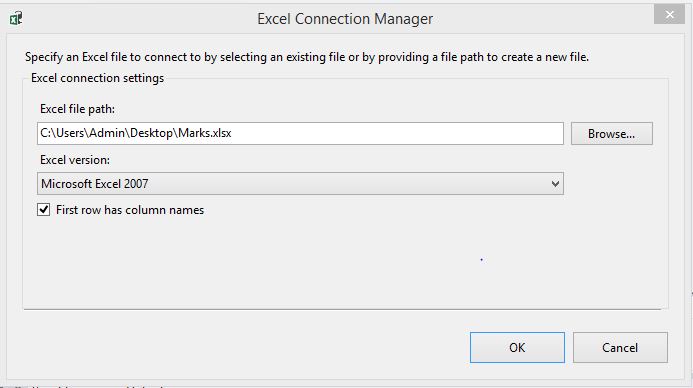
To do that we need to add an EXCEL source inside the dataflow task. When creating the “EXCEL connection manager”, I will un-tick the “First row as column names”, because this a vertical table and if I don’t do that it will end up taking the table values as column names. 

Then we have to configure the EXCEL source to get the Subject table only. We can use both methods to do this, I’m going to use the SQL command method as we discussed earlier. 

Then the preview and the columns will look like below.

As you can see in the columns I have renamed F1 as Category, since that column is representing the column names which are Subjectcode and Subjectname of our Subject table.

Then I’m going to connect a Unpivot tool to the EXCEL source.

I’ll configure the Unpivot table as below.

I select the F2, F3 and F4 from the input columns and named the destination column as “Value” and Pivot key value column name as “Measure”.

If we load this data to a destination that output will look like below.

Now we are going to Pivot the out of Unpivot but before that we have to sort the output of Unpivot.

Use sort tool and sort by “Measure” column.

After sort the Unpivot output it will look like below.

The important thing in about output is the “Measure” column. As you can see it maps the values between Subjectode and Subject name. For example, MAT01 and Maths from “Value” have same “Measure” as F2.

Then add a Pivot tool and configure it as below.

Set Pivot key is “Category”, Set key is “Measure” and Pivot value is “Value” and click ok.

By default, it sets only the “Measure” column which holds the mapping as pivot default output. With this mapping we going to create the Subjectcode and Subjectname as output columns. For that right click on the Pivot tool and go to Show Advanced Editor. After that go to Input and output properties and select Input columns in Pivot default input and get the LineageID of “Value” column. Then click the Pivot default output and you can see there is only “Measure” as output. Click on the Pivot default output and create columns for Subjectcode and Subjectname. Subjectcode and Subjectname columns should have “Value” column LineageID as Source column in Custom Properties. Then add the Pivot key values of Subjectcode as “Subjectcode” which is exactly as same as in the EXCEL sheet. Also do the same for subjectname as well.

Now if we get the result to a destination table we’ll get below output.

Still we are not finished. Now we have to join this with the Marks table in the EXCEL sheet. To do that first we have to create another EXCEL connection manager and configure it to get the same EXCEL sheet but with First row has column name ticked.

And then we need to follow the steps in the Excel loading Example 2, method 1 or method 2 to get the Marks table. After that we are going to use the Merge Join tool to join the Marks table with the Subject table which we created so far. But before that again we have to use Sort tool and sort the Subjectcode column which is the common column for both Marks and Subject tables. After configuring the sort tools, we have to connect the both tools output to the Merge join tool. First we have to join the sort output of Marks table because we are going to use left join to join the tables and the left table should be the Marks table. After connecting the Marks table select the Merge join left input from the Merge join tool and then connect the sort output of Subject table.

Next double click on the merge tool again and choose the final output columns you need. In this case I choose StudentID, Subjectcode, Subjectname and Marks as below.

Then set up the destination and execute, we can get the output.

The final result will be as given below.

This is the end of  1st part of EXCEL and SQL Server Integration Services.